This is the third in an occasional series of posts exploring OpenSCAD modeling techniques. The library described in this post can be found in the github repo.
In this article I'm going to discuss some approaches for creating organic-looking curved objects in OpenSCAD, and some general patterns for functions and modules to create non-built-in solids and operations.
OpenSCAD is widely used to create geometrically simple 3D models. Many very useful objects can be formed from unions and differences of simple solids--mounting brackets, wheels, shims, hooks, and other objects that might be found (or to be more direct, might break) within common consumer products. OpenSCAD is great at modeling a replacement for a $0.05 plastic part that saves you having to spend $50 replacing the thing it broke off from. But this post is about looking deeper, at the considerable power available if you're willing to spend a little time getting used to its idiosyncratic syntax. Specifically, I'm going to describe a technique for building curved polyhedra, with one eye towards procedural model generation.
OpenSCAD has two types of procedural abstractions: functions and modules. Functions are pure, side-effect-free transformations of input data (numbers, strings, booleans, arrays, undef) to output data. Modules are code blocks that may or may not take arguments and may or may not render objects as a side effect. They have no return value. One of the defining restrictions of this division is that there is no way to query the properties of a shape that has been rendered.
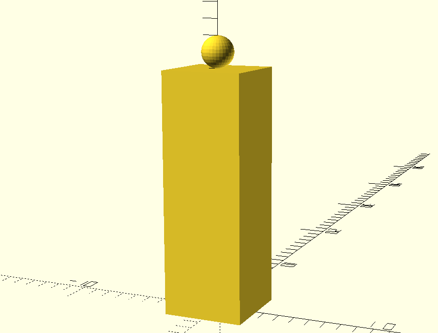
For instance, let's say I want a module that draws a sphere on top of a cube. Using the children
function described in my last post, I might think of something like this:
module sphere_on_cube(sphere_radius) {
  children(0); // this is the cube
  translate([0, 0, <figure out how tall the cube is>]) {
    sphere(sphere_radius);
  }
}

sphere_on_cube(1) cube([5, 5, 15]);
But this will never work, because rendered models are not available in code. Modules
like cube and children do not have return values; only side effects. There is simply
no way to query the properties of an object if all you have is the module that will render it.
Instead, for code where you want to make decisions based on the properties of objects,
you need to delay the rendering step until the very end of your pipeline, and operate on
data until you're ready to render everything. One correct (but silly) way to write the
sphere_on_cube module above would be to use a function to generate the location of
the sphere, based on the dimensions of the cube:
function sphere_translation(cube_dimensions, radius) = [
  0, 0, cube_dimensions[2] + radius
];

module sphere_on_cube(cube_dimensions, sphere_radius) {
  translate([-cube_dimensions[0] / 2, -cube_dimensions[1] / 2, 0]) {
    cube(cube_dimensions);
  }
  translate(sphere_translation(cube_dimensions, sphere_radius)) {
    sphere(sphere_radius, $fn=30);
  }
}

cube_dimensions = [5, 5, 15];

sphere_on_cube(cube_dimensions, 1);
This is a contrived example--it's not really necessary to define a function just to extract
the cube height--but it illustrates the pattern of representing objects within the code as
numeric arrays of data (the cube_dimensions) and rendering them as late as possible
so that other code (sphere_translation) can operate on the numeric representation. This
pattern is crucial for rendering more complex objects. For instance, let's look at the
problem of rendering a Bézier curve.
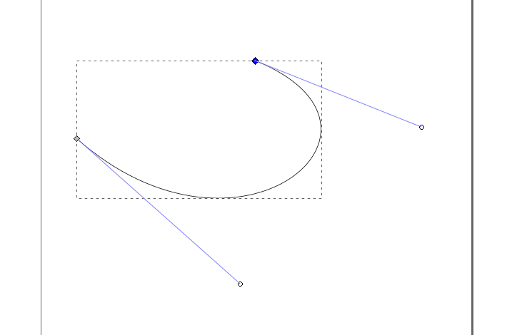
Bézier curves are parametric curves that will be familiar to anyone who has used a vector-based drawing program like Inkscape or Illustrator. They are curved lines that can be adjusted by moving "control points" which are usually represented as handles coming off the ends of the line segments.
Representing a shape like this in OpenSCAD presents some challenges. It can't be constructed
with simple boolean operations on builtin polygons. It's also concave, which presents difficulties
using simple hull operations, which take a convex hull. If we try to make a curve by taking the hull
of four spheres in a curved line:
sphere_points = [
  [0, 0, 0],
  [1, 1, 0],
  [1, 2, 0],
  [0, 3, 0]
];

hull() {
  for (point=sphere_points) {
    translate(point) sphere(1);
  }
}
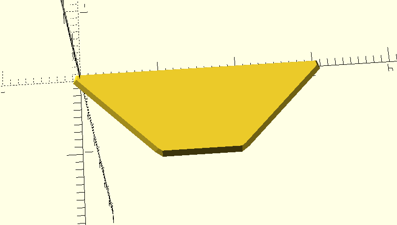
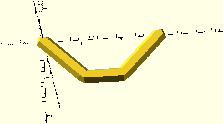
we lose the concavity of the shape we wanted, and instead get a convex blob. Instead, we can use a module that creates piecewise hulls of neighboring spheres to form a line:
module piecewise_join(points) {
  for (n=[1:len(points) - 2]) {
    hull() {
      translate(points[n-1]) children(0);
      translate(points[n]) children(0);
    }
    hull() {
      translate(points[n+1]) children(0);
      translate(points[n]) children(0);
    }
  }
}

sphere_points = [
  [0, 0, 0],
  [1, 1, 0],
  [1, 2, 0],
  [0, 3, 0]
];

piecewise_join(sphere_points) sphere(0.2);
Now we have a nice, if not very smooth, concave line.
Using the "render last" pattern described above, this piecewise_join function belongs at
the end of a pipeline, after we've determined the points along the line. The next task is
to determine where those points should go.
The central innovation in Bézier curves is the use of a small number of control points to specify a more complicated line. An excellent introduction is Pomax's Primer on Bézier Curves-- it's what I used as a reference to make most of these modules, along with ScratchaPixel's Bézier Curves and Surfaces: the Utah Teapot. Instead of attempting to reproduce those resources here, I'm just going to work through an example and then describe a couple of techniques for turning it into functions.
The Bézier equation is simply a way to interpolate values between a set of control points.
It uses a variable t which can be thought of as the "percentage along the line". At t=0,
the point that comes out of the Bézier function is exactly the first control point, because
that is the beginning of the line, and t=0 means "the position when you have traveled 0% of
the distance along the line". Likewise, when t=1, the point that comes out of the Bézier
function is exactly the last control point, because the last control point is where the line
ends, and t=1 means "the position when you have traveled 100% of the distance along the line."
By using values of t between 0 and 1, we can generate points along the line at whatever intervals
we want.
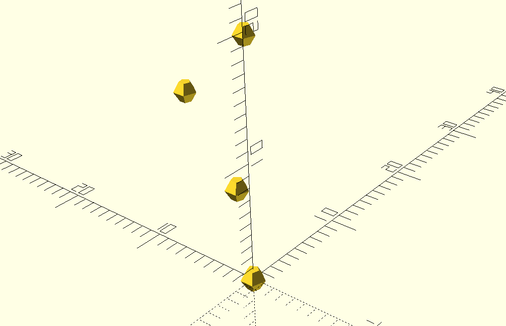
Let's define some control points so that there's something more concrete to use as an example.
control_points = [
  // this is the start of the curve
  [0, 0, 0],
  // this point influences the curve, but the curve does not
  // pass through it
  [3, 4, 5],
  // this point influences the curve, but the curve does not
  // pass through it
  [6, 12, 10],
  // this is the end of the curve.
  [9, 8, 15],
];

module draw_points(points) {
  for (point = points) {
    translate(point) children(0);
  }
}

draw_points(control_points) sphere(1);
When calculating a point between the beginning and end, we calculate each of the coordinates
separately. Let's take the halfway point along the curve: t=0.5. To find the coordinates
of the point along the curve at t=0.5, we use
halfway_point = [
  // find the x-coordinate at t=0.5, using the x-values of
  // the control points
  bezier_coordinate(0.5, [0, 3, 6, 9]),
  // find the y-coordinate at t=0.5, using the y-values of
  // the control points
  bezier_coordinate(0.5, [0, 4, 12, 8]),
  // find the z-coordinate at t=0.5, using the z-values of
  // the control points
  bezier_coordinate(0.5, [0, 5, 10, 15]),
];
So how do we define the bezier_coordinate function? To borrow from Pomax's excellent tutorial, the
bezier_coordinate function is represented as:

This specifies a polynomial with a number of terms equal to the number of control points. To
start calculating the x-coordinate of our point at t=0.5, we have:
// The binomial terms are the coefficients of the expansions of
// (1+x)^n, also known as Pascal's Triangle
b_terms = [
     [1],     // n = 0
   [1, 1],    // n = 1
 [1, 2, 1],   // n = 2
[1, 3, 3, 1]  // n = 3
];

// x-values of the control points, in order
weights = [0, 3, 6, 9];

// n from Pascal's Triangle where the number of coefficients is the
// same as the number of our control points
n = 3
term_0 = weights[0] * b_terms[3][0] * pow((1 - t), (n - 0)) * pow(t, 0)
//             0    *      1        *         0.5^3         *  0.5^0
//             0    *      1        *         0.125         *  1
//                                0
term_1 = weights[1] * b_terms[3][1] * pow((1 - t), (n - 1)) * pow(t, 1)
//             3    *      3        *         0.5^2         *  0.5^1
//             3    *      3        *         0.25          *  0.5
//                               1.125
term_2 = weights[2] * b_terms[3][2] * pow((1 - t), (n - 2)) * pow(t, 2)
//             6    *      3        *         0.5^1         *  0.5^2
//             6    *      3        *         0.5           *  0.25
//                               2.25
term_3 = weights[3] * b_terms[3][3] * pow((1 - t), (n - 3)) * pow(t, 3)
//             9    *      3        *         0.5^0         *  0.5^3
//             9    *      3        *         0.5           *  0.25
//                               3.375
x = term_0 + term_1 + term_2 + term_3
If we wanted to implement this function in a naive way, assuming that we would always have four control points, we could just use a long expression:
function bezier_coordinate(t, weights) = (
  (weights[0] * 1 * pow((1 - t), (3 - 0)) * pow(t, 0)) +
  (weights[1] * 3 * pow((1 - t), (3 - 1)) * pow(t, 1)) +
  (weights[2] * 3 * pow((1 - t), (3 - 2)) * pow(t, 2)) +
  (weights[3] * 1 * pow((1 - t), (3 - 3)) * pow(t, 3))
);
Then we can write a small function to take a value of t and a set of
exactly four control points, and calculate the point on the curve for
the given value of t.
function bezier_point(t, control_points) =
  [
    bezier_coordinate(t, [
      control_points[0][0],
      control_points[1][0],
      control_points[2][0],
      control_points[3][0]
    ]),
    bezier_coordinate(t, [
      control_points[0][1],
      control_points[1][1],
      control_points[2][1],
      control_points[3][1]
    ]),
    bezier_coordinate(t, [
      control_points[0][2],
      control_points[1][2],
      control_points[2][2],
      control_points[3][2]
    ])
  ];
These aren't great--it would be nice to be able to use different numbers
of control points--but there's enough here to glue it all together and see
some results. In most languages, we would be able to use a for loop to build
up a list of points, but in OpenSCAD arrays are immutable, so we need to use
a comprehension:
function bezier_curve_points(control_points, num_points) =
  [for (t=[0:1 / num_points:1]) bezier_point(t, control_points)];
So now we can look at the curve and make sure it works:
function bezier_coordinate(t, weights) = (
  (weights[0] * 1 * pow((1 - t), (3 - 0)) * pow(t, 0)) +
  (weights[1] * 3 * pow((1 - t), (3 - 1)) * pow(t, 1)) +
  (weights[2] * 3 * pow((1 - t), (3 - 2)) * pow(t, 2)) +
  (weights[3] * 1 * pow((1 - t), (3 - 3)) * pow(t, 3))
);

function bezier_point(t, control_points) =
  [
    bezier_coordinate(t, [
      control_points[0][0],
      control_points[1][0],
      control_points[2][0],
      control_points[3][0]
    ]),
    bezier_coordinate(t, [
      control_points[0][1],
      control_points[1][1],
      control_points[2][1],
      control_points[3][1]
    ]),
    bezier_coordinate(t, [
      control_points[0][2],
      control_points[1][2],
      control_points[2][2],
      control_points[3][2]
    ])
  ];

function bezier_curve_points(control_points, num_points) =
  [for (t=[0:num_points]) bezier_point(
    t * (1 / num_points), control_points
  )];

module draw_points(points) {
  for (point = points) {
    translate(point) children(0);
  }
}
module piecewise_join(points) {
  for (n=[1:len(points) - 2]) {
    hull() {
      translate(points[n-1]) children(0);
      translate(points[n]) children(0);
    }
    hull() {
      translate(points[n+1]) children(0);
      translate(points[n]) children(0);
    }
  }
}

control_points = [
  [0, 0, 0], // this is the start of the curve
  [3, 4, 5], // this point influences the curve, but the curve does not pass through it
  [6, 12, 10], // this point influences the curve, but the curve does not pass through it
  [9, 8, 15], // this is the end of the curve.
];

draw_points(control_points) sphere(1);
piecewise_join(bezier_curve_points(control_points, 10)) sphere(0.2);
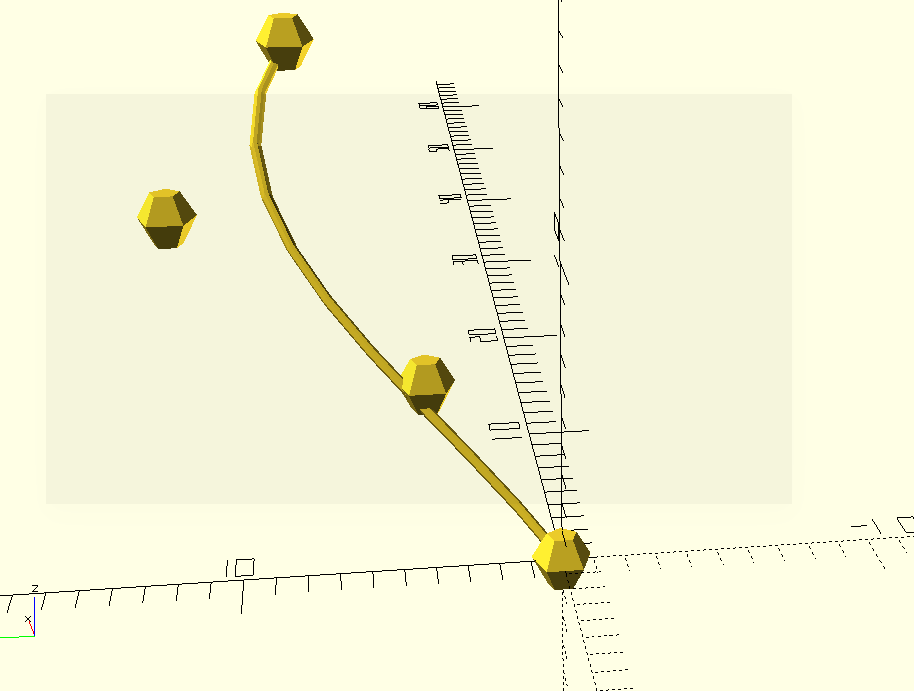
With moderately complicated things like this, it's helpful to get a simple,
representative case like this working quickly, then generalize it. As I mentioned
before, it would be nice to be able to specify an arbitrary number of control points.
To do that, we need to modify the bezier_coordinate and bezier_point functions.
For simplicity, we'll use a lookup table for the binomial coefficients, and leave the function to generate them as an exercise for the reader.
binomial_terms = [
      [1],               // n = 0
     [1, 1],             // n = 1
    [1, 2, 1],           // n = 2
   [1, 3, 3, 1],         // n = 3
  [1, 4, 6, 4, 1],       // n = 4
 [1, 5, 10, 10, 5, 1],   // n = 5
[1, 6, 15, 20, 15, 6, 1] // n = 6
];
We'll start by updating the bezier_coordinate function. In other languages, we could
use a for loop over the terms of the expression (because the number of terms depends
on the number of control points) with an accumulator variable to hold the running total,
like this version in javascript:
const pow = Math.pow;

function bezier_coordinate(t, weights) {
  const n = weights.length - 1;
  const binomial_row = binomial_terms[n];
  let total = 0;
  const a = 1 - t;
  const b = t;
  for (term = 0; term < weights.length; term++) {
    const a_pow = n - term;
    const b_pow = term;
    total += (
      weights[term] * binomial_row[term] *
      pow(a, a_pow) * pow(b, b_pow)
    );
  }
}
This works in Javascript, but in OpenSCAD is a functional language; variables can't
be reassigned at runtime. Instead of using += with an accumulator variable, we need
to use recursion to acheive the same effect. This pattern will be especially familiar
to anyone who has used Lisp or other functional languages.
function bezier_coordinate(t, weights, term=0, total=0) =
  let (
     n = len(weights) - 1,
     binomial_row = binomial_terms[n],
     a = 1 - t,
     b = t,
     a_pow = n - term,
     b_pow = term
  )
  (term > n ? total :
    bezier_coordinate(
      t,
      weights,
      term + 1,
      (
        total + (weights[term] * binomial_row[term]
        * pow(a, a_pow) * pow(b, b_pow))
      )
    )
  );
At each iteration of the recursion, we check the term parameter to see if we've finished
evaluating all of the terms. If so, we return the total. If not, we evaluate the current term
and then call the function again for the next term, adding the value of this term to the
running total. This is how every function that accumulates a value in OpenSCAD has to work.
For the bezier_point function, all we really need is to generalize it to select the nth
element from each of the control points, to gather the weights for a particular coordinate.
For that, we can use list comprehensions similar to those in the bezier_curve_points function:
function bezier_point(t, control_points) =
  [
    bezier_coordinate(t, [for (point = control_points) point[0]]),
    bezier_coordinate(t, [for (point = control_points) point[1]]),
    bezier_coordinate(t, [for (point = control_points) point[2]]),
  ];
Now we can test again, with our generalized version.
binomial_terms = [
      [1],               // n = 0
     [1, 1],             // n = 1
    [1, 2, 1],           // n = 2
   [1, 3, 3, 1],         // n = 3
  [1, 4, 6, 4, 1],       // n = 4
 [1, 5, 10, 10, 5, 1],   // n = 5
[1, 6, 15, 20, 15, 6, 1] // n = 6
];
function bezier_coordinate(t, weights, term=0, total=0) =
  let (
     n = len(weights) - 1,
     binomial_row = binomial_terms[n],
     a = 1 - t,
     b = t,
     a_pow = n - term,
     b_pow = term
  )
  (term > n ? total :
    bezier_coordinate(
      t,
      weights,
      term + 1,
      (
        total + (weights[term] * binomial_row[term]
        * pow(a, a_pow) * pow(b, b_pow))
      )
    )
  );
function bezier_point(t, control_points) =
  [
    bezier_coordinate(t, [for (point = control_points) point[0]]),
    bezier_coordinate(t, [for (point = control_points) point[1]]),
    bezier_coordinate(t, [for (point = control_points) point[2]]),
  ];

function bezier_curve_points(control_points, num_points) =
  [for (t=[0:num_points]) bezier_point(
    t * (1 / num_points), control_points
  )];

module draw_points(points) {
  for (point = points) {
    translate(point) children(0);
  }
}
module piecewise_join(points) {
  for (n=[1:len(points) - 1]) {
    hull() {
      translate(points[n-1]) children(0);
      translate(points[n]) children(0);
    }
  }
}

module bezier_curve(control_points, number_of_sections) {
  piecewise_join(
    bezier_curve_points(control_points, number_of_sections)
  ) children(0);
}

control_points = [
  [0, 0, 0],
  [3, 4, 5],
  [6, 12, 10],
  [9, 8, 15],
];

draw_points(control_points) sphere(1);
bezier_curve(control_points, 10) sphere(0.2);
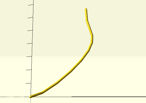
Now we are not restricted to cubic curves, so we can use the number of control points appropriate to the line we want to draw.
So what can we do with a custom bézier curve module? Well, since we have access to all the curves' points in code, let's try to use that in a way that would be difficult in a GUI.
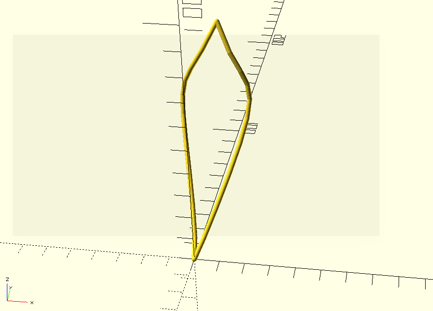
For instance, we can take a kind of half-leaf-shaped curve:
use <./lib/bezier.scad>;

LEAF_EDGE_CONTROL_POINTS = [
  [0, 0, 0],
  [2, 20, 0],
  [24, 80, 60],
  [16, 40, 40],
  [0, 60, 75]
];

bezier(LEAF_EDGE_CONTROL_POINTS, 10), sphere(1);
Notice that this curve uses five control points to specify a slightly more complex curve than would be possible with only four. As we'll see, it's easy to use curves with different numbers of control points in the same model.
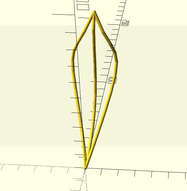
If we want to make the whole leaf shape, all we have to do is mirror the curve.
use <./lib/bezier.scad>;

LEAF_EDGE_CONTROL_POINTS = [
  [0, 0, 0],
  [2, 20, 0],
  [24, 80, 60],
  [16, 40, 40],
  [0, 60, 75]
];

bezier(LEAF_EDGE_CONTROL_POINTS, 10) sphere(1);
mirror([1, 0, 0]) bezier(LEAF_EDGE_CONTROL_POINTS, 10) sphere(1);
We can add a line in the middle, by adding another set of control points with the same first and last points:
use <./lib/bezier.scad>;

LEAF_EDGE_CONTROL_POINTS = [
  [0, 0, 0],
  [2, 20, 0],
  [24, 80, 60],
  [16, 40, 40],
  [0, 60, 75]
];

LEAF_CENTER_CONTROL_POINTS = [
  [0, 0, 0],
  [0, 20, 0],
  [0, 80, 10],
  [0, 40, 55],
  [0, 60, 75]
];

bezier(LEAF_EDGE_CONTROL_POINTS, 10) sphere(1);
bezier(LEAF_CENTER_CONTROL_POINTS, 10) sphere(1);
mirror([1, 0, 0]) bezier(LEAF_EDGE_CONTROL_POINTS, 10) sphere(1);
So far, we've just been using curves in the same way we did before. But if we generate the curve points first, we can use them in further shapes. The shape looks something like a leaf; we can add veins by connecting points from the center curve to points on the outer curves. By generating the outer curve points and the center curve points, we can use a for loop to match them, and generate an intermediate control point that will give us a nice curve.
use <./lib/bezier.scad>;

LEAF_EDGE_CONTROL_POINTS = [
  [0, 0, 0],
  [2, 20, 0],
  [24, 80, 60],
  [16, 40, 40],
  [0, 60, 75]
];

LEAF_CENTER_CONTROL_POINTS = [
  [0, 0, 0],
  [0, 20, 0],
  [0, 80, 10],
  [0, 40, 55],
  [0, 60, 75]
];

SAMPLES = 20;

module leaf_half() {
  // render the outside edge of the leaf
  bezier(LEAF_EDGE_CONTROL_POINTS, SAMPLES) sphere(1);
  // get the [x, y, z] coordinates of the points that
  // make up the curve
  edge_points = bezierPoints(LEAF_EDGE_CONTROL_POINTS, SAMPLES);
  // get the [x, y, z] coordinates of the points that make up the
  // center line
  center_points = bezierPoints(LEAF_CENTER_CONTROL_POINTS, SAMPLES);
  // We want the veins to slant up from the center to the outside of
  // the leaf, so we match the point 3 on the center line with point
  // 6 on the outside edge, point 4 in the center with 7 on the edge,
  // and so on until we get to the last point on the edge
  for (i=[6:SAMPLES]) {
    ep = edge_points[i];
    cp = center_points[i - 3];
    // We use 3 points to define the curve for the vein. The first
    // point is a point on the edge, the last point is on the
    // center, and the middle point is halfway between and skewed a
    // little toward the bottom and "underside" of the leaf, to give
    // the vein a nice curve.
    vein_points = [
      ep,
      [
        ((ep[0] + cp[0]) / 2),
        ((ep[1] + cp[1]) / 2),
        ((ep[2] + cp[2]) / 2) - 5
      ],
      cp
    ];
    bezier(vein_points, SAMPLES) sphere(1.2);
  }
}


// to render the whole leaf, we render half the leaf, mirror it,
// and render the middle line just once.
module leaf() {
  leaf_half();
  mirror([1, 0, 0]) leaf_half();
  bezier(LEAF_CENTER_CONTROL_POINTS, SAMPLES) sphere(2);
}
leaf();
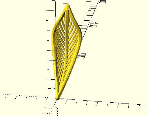
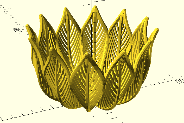
Finally, given the leaf function, we can render a series of leaves rotated
about the Z-axis, creating the bowl from the beginning of this post:
LEAVES = 12;
for (i=[0:360 / LEAVES: 360]) {
  rotate([0, 0, i]) leaf();
}
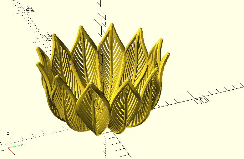
One of OpenSCAD's great strengths is the flexibility of defining models in code.
With access to the geometry of your model, you can express domain-specific relationships
like the veins on a leaf in a durable way. In this example, the relationship between
the center of the leaf and the edge that defines the veins would allow us to modify
the leaf shape without having to adjust them. This also demonstrates the use of recursive
functions and the "render-last" pattern that works best for assembling complex models.
Finally, this is an example of a parametric yet organic-looking shape. Look for future
posts to explore the potential for Bézier surfaces and the polyhedron module.
The code in this post is loosely based on examples from my bezier-scad library. Check it out if you want to see more!